The Julia Fractals

_{Created for the University of Alberta CMPUT 229 Architecture course}

Information

This lab introduces the floating-point registers of the RISC-V architecture as well as GLIR, a graphics library for RISC-V (originally GLIM for MIPS) built at the University of Alberta. These tools will be used to perform arithmetic on complex numbers and create a RISC-V program that renders Julia fractals on the terminal.

Complex Numbers

A complex number is composed of two parts: a real part and an imaginary part. Consider the complex number $c$, where $c = 4 + 5i$. The real part of $c$ has a value of $4$ and the magnitude of the imaginary part has a value of $5$. $i$ is a special number called the imaginary unit because it satisfies the equality $i^2 = -1$. Imaginary numbers follow the standard arithmetic rules that you are already familiar with on real numbers: e.g. the sum of imaginary numbers $2i$ and $3i$ is $5i$.

Complex numbers are made up of two separate components (real numbers and imaginary numbers) and can be visualized on a plane. Similar to how we plot the point $(x, y)$ on the $x$-$y$ plane, we plot complex numbers on the complex plane. The complex plane has a real-axis and an imaginary-axis, much like the familiar $x$-axis and $y$-axis for real numbers.

The absolute value of a complex number is the distance between the origin and the point defined by its real and imaginary values. Given a complex number $c = a + bi$ According to Pythagoras' theorem, $|c| = \sqrt{a^2 + b^2}$, where $a$ is the real value and $b$ is the magnitude of the imaginary value.

Julia Sets

The Julia sets are sets of complex numbers defined by whether or not their absolute values tend to infinity when a function is repeatedly applied to them. To compute a Julia set, one must provide the complex plane (in which a computer determines each point's membership in the set), and a constant complex number used as part of this computation. Changing this constant value will give varying sets. This lab renders a single Julia fractal — a visualization of a single Julia set on a complex plane — and therefore works with a single constant number. The function that defines whether or not a complex number belongs to a Julia set is:

\begin{eqnarray} z_0 &=& z \\ z_n &=& z_{n-1}^2 + c\\ \end{eqnarray}

where $z$ is the complex number whose membership in the Julia set is being determined, and $z_n$ indicates the complex number after $n$ iterations of the function. $c$ is a constant complex number: for this lab, $c = -0.8 + 0.156i$. The complex number $z$ belongs to a Julia set if, as $n$ approaches infinity, $|z_n|$ does not tend to infinity. If, however, $|z_n|$ is not bounded and tends to infinity as $n$ approaches infinity (diverges), then $z$ does not belong to the Julia set.

Suppose the membership of some complex number $z$ in the Julia set with constant $c = -0.8 + 0.156i$ is being determined. The computations would follow these steps:

$\begin{eqnarray} z_0 &=& z &=& z &=& z \nonumber \\ z_1 &=& z_0^2 + c &=& z^2 + c &=& z^2 + c \nonumber \\ z_2 &=& z_1^2 + c &=& (z^2 + c)^2 + c &=& z^4 + 2cz^2 + c^2 \nonumber \\ \cdots \nonumber \end{eqnarray} $

Note that each $z_k$ is indeed simplified to a complex number of form $c = a + bi$ because $i = \sqrt{-1}$, and $i^2 = -1$.

It seems to be a problematic task to compute $|z_k|$ for each of the $z_n$ complex numbers and determine if the series diverges (tends to infinity as $n$ goes to infinity). This is obviously not feasible. It is, however, known that if any $z_k$ exists such that $|z_k| >= 2$, the complex number $z$ will diverge. In other words, when some $|z_k|$ exceeds the value of 2, the program can conclude that $z$ does not belong to the set.

Calculating the square root in RISC-V assembly is computationally expensive. Fortunately, given that $|c| = \sqrt{r^2 + i^2}$, squaring both sides gives $|c|^2 = r^2 + i^2$. Thus, it is less computationally expensive to compute the square of the absolute value of $z_k$, and then compare this value with $4$ instead of $2$.

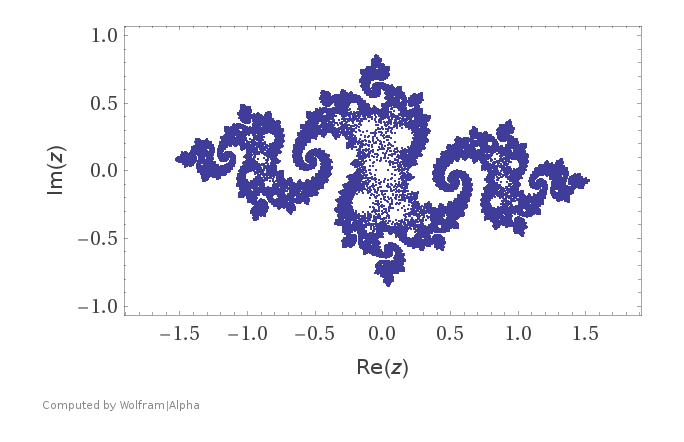
The following is an image generated by Wolfram|Alpha depicting the membership in the Julia set of all complex numbers. Here, the purple points indicate complex numbers that belong to the set, whereas the white points do not. Complex numbers (points in this graph) that do not belong to the set are said to have escaped because they 'escape' the bound that would otherwise make them a member of the set.

Julia Animations

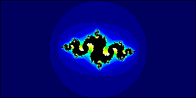
Suppose there is a complex number that does not belong to our Julia set. The coloured rendering of a fractal requires the escaping iteration of the number. A given $z$ may escape on the first few iterations or it may not escape until the trillionth iteration. Artistic renditions of Julia sets colour the points on a Julia fractal based upon the iteration they escaped. This animation produced by joshig1983 renders a mesmerizing zoom of a Julia fractal. The colours indicate how many iterations it took a particular point to escape. Julia fractals can be computed to tremendous precision; they are limited only by the computing power and precision of the architecture.

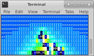
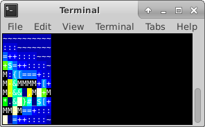
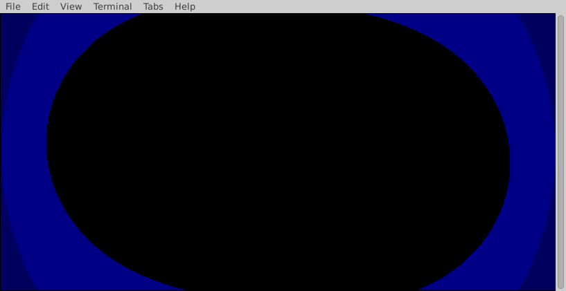
As another example, consider the animation below. In this animation, all black regions belong to the Julia set. Here, the different shades of colour indicate when a region of complex numbers escapes. The first frame of the .gif illustrates (in very dark blue) the sections of complex numbers that escaped in only one iteration. The second frame includes the section of complex numbers where it took two iterations to escape, and so on. The animation was set to illustrate all sections that escape within 25 iterations. Observe that the colour scheme goes from dark to light to produce a smooth, aesthetically appealing fractal.

What would the animation look like if it were left to compute further iterations for the regions that did not escape? Indeed, some in-set regions (black) of this animation would have escaped and be coloured.

GLIR - the RARS Graphics Library

This assignment is to be written in RISC-V and uses graphics to display the results of the computation. Graphics will be handled with GLIR, a Graphics LIbrary for RISC-V built at the University of Alberta. For the purpose of this assignment only the Screen Updates section is relevant. This section details the printString method that will be used to print colour-coded characters to the screen. printString takes in the address of the null-terminated string to print, as well as the terminal row and terminal column to print to. In the coordinate system of terminal screens, the position (0,0) is located at the top left corner (as detailed in the GLIR documentation). Your solution will determine what complex number each tile on the terminal maps to and assign it a character and colour, then print it. The background colour of each character will be set using setColor. Note that in the .gif above, the character was set to a space on every tile (for illustrative purposes).

Coordinate systems

There are two coordinate systems in use for this assignment. Translation between the two systems is handled by a function called map_coords (which stands for 'map coordinates'). The code for this function is provided to you in a common file. Regardless, it is important to understand what is happening because writing the code for set_size is part of the solution to the assignment. The function set_size gives map_coords the information that it needs for the mapping between the two coordinate systems. An empty implementation of set_size will still produce a fractal if the other functions are correct, but correct mapping requires set_size to be complete.

Complex Coordinates

Julia fractals are displayed on the complex plane. A complex plane can be represented as a 2-tuple of a real interval and an imaginary interval. The notation (real_interval, imaginary_interval) represents intervals for both the real part and imaginary part of complex numbers. Both intervals are represented by the notation [min, max] - therefore a complex plane can be represented as:
([min_real, max_real), (min_imaginary, max_imaginary])

The .gif animation above was generated on the complex plane([-2.0, 2.0), (-1.0, 1.0]). A Julia fractal is simply a rendition of the Julia set on some complex plane. The complex plane ([-20.0, 20.0), (-10.0, 10.0]) would show the same animation as above, except ten times zoomed out. Alternatively, it's also possible to zoom in on some part of the fractal. If the dimensions of the terminal are kept constant, but the intervals of the complex plane are narrowed, the fractal would be more detailed.

Terminal Coordinates

The terminal screen is made up of tiles, with each tile having an integer coordinate (row, col). The terminal spans [0, # of rows] in the vertical position and [0, # of columns] in the horizontal position. The row position represents the vertical distance from the top of the screen. The column, or col, is the horizontal distance from the left of the screen. This is a construct of terminal windows that is preserved by the GLIR library because it is a common graphics standard, despite being the opposite of the mathematical standard to put the horizontal element first in a coordinate.

Translation

The common file will setup user input for you, so at the start of your program the user will be prompted to enter the dimensions of the terminal as well as the complex plane being rendered. Recall that we can only determine if a point belongs to a Julia set if the point is a complex number. Since the fractal is being displayed on the terminal, how can each terminal tile be mapped to a complex number? This is taken care of you by the common file function map_coords, however, you are responsible for programming the set_size subroutine. This function will calculate the "step sizes" given the user input. These step sizes will evenly divide the given complex plane such that each tile on the terminal has a corresponding complex coordinate.

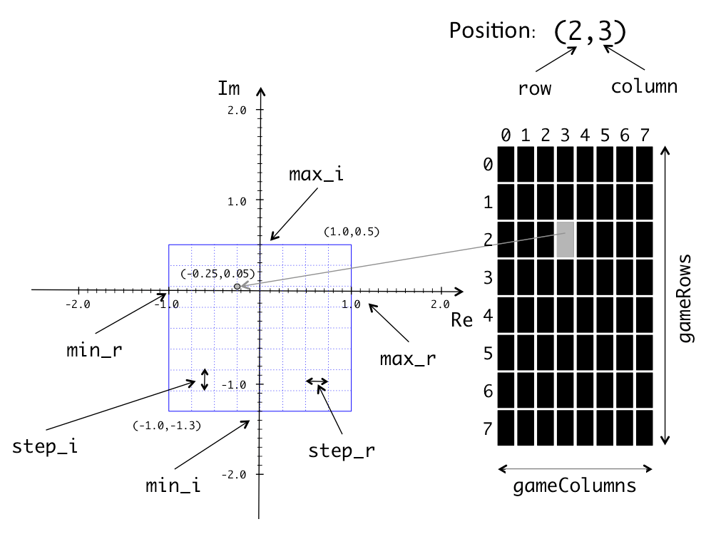
The figure below illustrates mapping for a display with $8 \times 8$ tiles that is to display the section of the complex plane defined by ([-1.0, 1.0),(-1.3, 0.5]). The bottom-left point of this section is (-1.0,-1.3) and the upper-right point is (1.0,0.5). The figure shows how the complex plane is divided into the same number of tiles as the display and how the tile (2,3) maps to the point (-.025,0.05) which is in the top-right corner of the corresponding tile in the complex plane. The figure also indicates the meaning of the values min_i, max_i, min_r, max_r, step_i, step_r, gameColumns, and gameRows. These values will be stored in memory locations previously allocated in the common.s file provided with this assignment.

In the following animation the terminal dimensions remain constant, but the portion of the complex plane that is rendered varies. To generate this animation, the program progressively renders smaller and smaller portions of the plane, focusing in on a small region in the top portion of the original image. As inspiration, this rendering was created using a solution to this assignment.

Floating-Point Registers

In addition to RISC-V's integer registers, there are other registers dedicated to handling floating-point operations. There are extensions to the base RISC-V architecture for operating on those registers. There are instructions to move values between the integer registers and the floating-point registers, as well as to translate binary values from integer format to floating-point format and vice versa. The solution to this assignment does not require an understanding of binary floating-point representations.

Precise numbers are required for the objective of the lab, therefore simple integer values won't do. Numbers with decimals can be represetend in binary in floating-point format. We can use single-precision floating-point values, which RISC-V stores in 32 bits, or double-precision floating-point values (64 bits). Since RARS does not support double-precision floating point values, this assignment operates with single-precision floating-point values.

Regular and Floating-Point Registers

RISC-V has integer registers (e.g. s3, t2, or s5) and floating-point registers (eg. ft0, fs1, or fa2). In the following lists, R[] denotes integer registers, while F[] denotes floating-point registers. rd, rs1, rs2 indicate which operand the respective register is. This section is adapted from this webpage based on RARS' documentation.

Transferring Values Between the Integer and Floating-Point Registers

The following instructions can be used to transfer values between regular registers and floating-point registers and to transfer values between memory and the floating-point registers. Note that the .s indicates that the instruction operates on at least one single-precision floating-point register.

• fmv.s.x F[rd], R[rs1]
• Copies the contents of integer register R[rs1] to single-precision floating-point register F[rd].
• fmv.x.s R[rd], F[rs1]
• Copies the contents of single-precision floating-point register F[rs1] to integer register R[rd].
• flw F[rd], offset(R[rs1])
• Loads 32 bits (1 word) from memory starting at the address provided by R[rs1] + offset, and stores it into F[rd].
• fsw F[rs2], offset(R[rs1])
• Stores the 32 bits found in F[rs2] into memory starting at the address provided by R[rs1] + offset.

Translating values

Instructions with floating-point operands require that values stored in those operands are in floating-point format. The below instructions will translate values for you. You must use these instructions to first transform values into floating-point format or integer format before performing operations on them.

• fcvt.s.w F[rd], R[rs1]
• Converts the word (integer) in R[rs1] to a float, and stores the result in F[rd]
• fcvt.w.s R[rd], F[rs1]
• Converts the float in F[rs1] to a word (integer), and stores the result in R[rd]

Floating-Point Arithmetic

The following floating-point arithmetic functions can be used to make perform arithmetic operations on double-precision floating-point values.

• fadd.s F[rd], F[rs1], F[rs2]
• F[rd] = F[rs1] + F[rs2]
• fsub.s F[rd], F[rs1], F[rs2]
• F[rd] = F[rs1] - F[rs2]
• fdiv.s F[rd], F[rs1], F[rs2]
• F[rd] = F[rs1] / F[rs2]
• fmul.s F[rd], F[rs1], F[rs2]
• F[rd] = F[rs1] * F[rs2]

Floating-Point Decisions

The following are floating-point conditional operators.

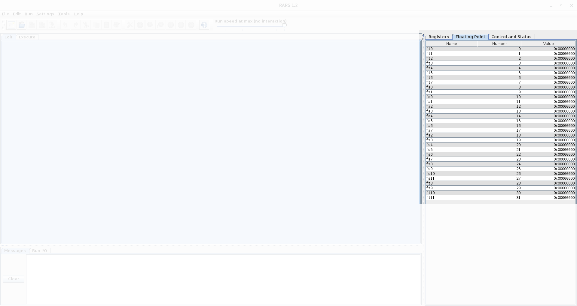
• feq.s R[rd], F[rs1], F[rs2]
• If F[rs1] is equal to F[rs2], it sets R[rd] to 1. It sets R[rd] to 0 otherwise.
• fle.s R[rd], F[rs1], F[rs2]
• If F[rs1] is less than or equal to F[rs2], it sets R[rd] to 1. It sets R[rd] to 0 otherwise.
• flt.s R[rd], F[rs1], F[rs2]
• If F[rs1] is strictly less than F[rs2], it sets R[rd] to 1. It sets R[rd] to 0 otherwise.

Available registers

The following is a picture of how RARS displays the values in floating-point registers - to see this area of RARS, click the Floating Point tab. There are 32 single-precision floating-point registers. This assignment uses only single-precision values.

Calling Conventions

Floating-point registers have a set of calling conventions similar to those found for the CPU registers: some are considered 'temporary' while others are 'saved' registers. The code provided to you in the common.s uses the following calling conventions for the floating-point registers.

• fa0 - fa7: Floating-point arguments.
• fa0 - fa1: Floating-point return values..
• ft0 - ft11: Temporary registers, not preserved across procedure calls.
• fs0 - fs11: Saved registers, preserved across procedure calls.

Strange errors will arise from your code if proper calling conventions are not followed. A common mistake from students is not saving callee-saved registers. For this assignment, any callee function must save registers fs0 - fs11, and then restore them before returning. For instance, if a function named caller has an instruction jal foo and foo modifies fs0, it is the responsibility of callee-function foo to save fs0, then restore it before a ret. Additionally, if function caller needs to ensure a caller-saved register such as ft0 is the same after a function call, it is the responsibility of function caller to save ft0 before a function call, then restore it. These same conventions must be followed with CPU caller-saved registers t and callee-saved registers s.

Assignment

The solution for this assignment consists of a RISC-V assembly file containing three functions to calculate the Julia function iterations and to print the results. The following are the specifications:

• set_size
• Sets the boundaries and the step sizes used by the map_coords function so that it properly maps coordinates to the desired portion of the complex plane. The set_size function must do the following:
• store the maximum imaginary value being rendered to the memory location max_i
• store the minimum real value being rendered to the memory location min_r
• compute the imaginary step size as the difference between the maximum and the minimum imaginary values divided by the number of rows in the screen and store this value in step_i
• compute the real step size as the difference between the maximum and the minimum real values divided by the number of columns in the screen and store this value in step_r
• Arguments:
• fa0 = maximum imaginary value being rendered: set max_i to this value.
• fa1 = minimum imaginary value being rendered
• fa2 = maximum real value being rendered
• fa3 = minimum real value being rendered: set min_r to this value.
• a0 = number of rows in the screen
• a1 = number of columns in the screen
• Return Values:
• None
• The memory locations max_i, min_r, step_i and step_r contain double floating-point values.
• The arguments for map_coords are in four floating-point registers and two integer registers. set_size will be called by the common file before your code needs to call map_coords.
• calculate_escape
  • Given a complex number $z$ and a maximum number of iterations, determine if $z$ escapes within the specified number of iterations. If $z$ does escape, also return the number of iterations it took. $z$ escapes at iteration $n$ if in the Julia function $|z_n|^2 \geq 4$. The complex number $z$ is represented by a pair $(r, i)$ where $r$ is the real portion and $i$ is the magnitude of the imaginary portion. The values of $r$ and $i$ are of type double and are stored in memory. The memory location for $r$ is z_x and the memory location for $i$ is z_y. The symbols z_x and z_y are available to calculate_escape. A pseudocode for calculate_escape is provided.
  • Arguments:
    • a0 = the max number of iterations.
    • z_x: .double = Initial real value of the complex number
    • z_y: .double = Initial imaginary value of the complex number
  • Return Values:
    • a0 = 'has_escaped', 1 if the number escaped before the max number of iterations, 0 if the number is in the set.
    • a1 = The number of iterations the algorithm went through before stopping. If the the max number of iterations was reached (a0 = 0) then this value is the value of a0, the max number of iterations.
• render
• This function uses two lists and three variables pre-defined in the common.s file to print each tile in the terminal screen. Before detailing the specification of render, lets review these pre-defined data structures (see the common.s file for their specification in assembly):
  • paletteSize: .word n
    the length of the symbol list and of the color lists; n is a non-negative integer
  • symbols: .asciz s1, s2, ..., sn
    list symbols stored in memory. Each symbol si is a null-terminated string.
  • colors: .byte c1, c2, ..., cn
    a list of color codes stored in memory. See the GLIR section in Hints on how to use setColor.
  • inSetColor: .byte 0
    a single color code to be used to print tiles whose values reach max iterations.
  • inSetSymbol: .asciz "M"
    a single char string to be used to print tiles whose values reach max iterations.
  All the characters above are null-terminated strings because a character is printed using the function print_string in GLIR. This is a GLIR design choice to enable the printing of sequences of escape characters.
• The render function must scan the entire display. For each tile in the display, render will execute the following steps:
  • invoke the function map_coords (provided in the common.s file) to determine which point in the complex plane that tile represents.
  • invoke calculate_escape to determine how many iterations that point takes to 'escape'. Pass to calculate_escape the max iterations value that render received as an argument
  • use the following algorithm to select the color and symbol to be printed for the tile based on the number of iterations returned by calculate_escape:
    • if the maximum number of iterations was reached:
      • select the inSetColor and
      • select the inSetSymbol
    • otherwise:
      • compute position = iterations % paletteSize where iterations is the number of iterations returned by calculate_escape and % is the modulus (or remainder of the division) between iterations and paletteSize. Recall that the RISC-V instruction rem is capable of calculating a modulus
      • select the color at position in the list colors
      • select the symbol at position in the list symbols
    • invoke the GLIR function setColor to set the selected color as background
    • invoke the GLIR function printString to print the selected symbol. Keep in mind the RISC-V calling conventions
• Arguments:
• a0 = number of Rows in the screen
• a1 = number of Columns in the screen
• a2 = max number of iterations
• Return Values:
• None

Invariants and Complications

• Your program must begin with the directive .include "common.s"
• Your program must support both printing the fractal using symbols and colors. Our marking scripts rely on the symbols you print, while our human graders rely on colors to understand your assignment when the marking scripts do not pass.
• The max size of screen that will be tested is 20 rows x 80 columns.
• The max number of iterations that will be test is 200.
• At the above maximums the max number of tiles that will belong to the set (reach max iterations) is about half of the screen.
• Floating-point operations are much slower than integer operations. Rendering a detailed fractal takes time. However, with the above invariants, any solution that takes longer than 10 seconds to render a scene will be considered failing.

Hints

• Make sure that your set_size and calculate_escape functions are working perfectly before you try to use them in the render function. Trying to debug them by using them in the render function can take much longer as the output can be very difficult to interpret if it is incorrect.
• Here is a pseudocode escape time algorithm to help you understand how to program your calculate_escape and render functions.
• Observe that map_coords returns the real part of the associated complex number in fa0 and the imaginary part in fa1, but calculate_escape takes in these arguments in the float-type memory locations z_x and z_y. It only makes sense, then, to store the results of map_coords into these memory locations before calling calculate_escape.
• Here is a complete example of what the output should look like for the following settings inputted at the start of the program:
  (rows, columns, max_i, min_i, max_r, min_r, iterations) = (20, 80, 1, -1, 2, -2, 25)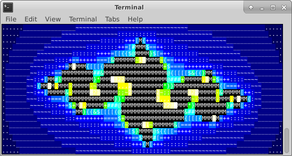
  

• And for (10, 40, 0.86, 0.84, -0.025, -0.065, 200)

• And for (10, 10, 0.5, -0.5, 1.5, 1, 100)

GLIR Functions for Printing Tiles

This section reviews how to use the two GLIR functions, setColor and printString, that you will be using to print coloured tiles and their associated strings (see the Assignment section). setColor takes in the arguments a0 = color code (byte), and a1 = 0 or 1, to set the background or foreground, respectively. For this assignment you must set a1 to 0 so that the tile is colored, and not the text that will be printed on it. a0 takes in a byte value, not an address. This is emphasized because printString takes in an address, and not a byte.

printString takes in the arguments: a0 = address of the null-terminated string to print, a1 = row to print to, and a2 = column to print to. In this assignment you will be loading the addresses of strings (see the symbols list in the common.s file) and passing in the row and column before calling this function. The symbols list is made up of .asciz strings, which means they end in a null (0x00) byte.

Your code should be structured in a procedural fashion. For each tile, you determine its corresponding complex number using map_coords. Then you determine if this point escapes, and if so, on what iteration. This information is then used to print the corresponding coloured tile using the functions in the GLIR library. Keep the RISC-V calling conventions in mind when using any function.

Common Issues

To debug RARS code, one must go through each instruction and determine if it is doing what it needs to be doing. This makes programming the assignment difficult because it is not always evident where the issue is. This section explores common errors and what the likely cause is.

• Bad address in data/stack read: Your program is accessing an address that does not belong to you. Check that the registers involved with loads and stores have not been overwritten. Also ensure that you are following RISC-V calling conventions - improper calling conventions will cause functions to overwrite registers that you may be using.
• Every tile is the exact same or the output does not match the fractal at all: Your render is likely working, but the problem may be in the implementation of your calculate_escape. Go over the code and see if it matches the provided pseudocode.
• Output fractal is only partially correct: The problem is likely in calculate_escape again. If the fractal is correct for only one row, or all rows but the last one, etc., then check the logic of your loops in render. Make sure all iteration registers are being appropriately set and incremented.
• Tile colours are incorrect or do not show: Check that you are using lbu - load byte unsigned, instead of lb to load from colors.
• Tile characters are correct but not colours (or vice-versa): Observe that colors is a list of bytes, whereas symbols is a list of single-char strings. This means that each string in symbols takes up two bytes (the character + a null byte).

Marking Guide

Here is a general idea of how the lab will be marked.

• Your submission will be run through about 8 tests using a semi-automatic marking script.
• Your results will be compared to our own solution and if they are equal your submission will pass every test automatically.
• There are deductions for submissions that print the correct escaped tile colors, but not the correct escaped tile symbols. There are much greater deductions for solutions that do not calculate or print the fractal itself correctly. If a submission fails to use GLIR functions properly and cannot render a fractal scene at all it will completely fail every test.
• Here is an example of a TA using the automatic marking script to mark a submission that has failed due to an improper implementation of calculate_escape and render.

There will be deductions for common mistakes in style, such as no function headers, no explanation of register usage, missing or few block comments, etc.

A copy of the marksheet is available here

Resources

• The in-class presentation of the lab.
• The in-lab presentation of the lab.
• The common.s file contains the GLIR library, and the framework that will call your methods to render the fractals. DO NOT SUBMIT THIS FILE WITH YOUR CODE.
• The animations that were included in this assignment description were made using some Octave and Bash scripts. These scripts are not part of the assignment and neither is creating animations. But curious students wanting to make some of their own are provided these resources here. It could be a nice way to test your solution.

Submission

Yous submission is a single file named julia.s. This file should only contain the functions belonging to the assignment. It should not include any GLIR functions, main method, or any portion of the common.s file provided in the Resources directory. Your solution MUST include the CMPUT 229 Student Submission License at the top of the file containing your solution. To create you solution you should edit the initial file already included in the Student_Solution folder. Make sure include your name in the appropriate place in the license text. The last commit/push prior to the deadline will be graded.