DISCLAIMER: This page contains math equations and images. If you cannot see either of them on this page, try loading the page on a different web browser.

Introduction

This lab introduces the Graphics Library for RISC-V (GLIR) and provides practice implementing algorithms in RISC-V assembly code. In particular, you will be implementing the A* (A-star) algorithm for solving pathfinding problems.

Background

Pathfinding algorithms are designed to find the shortest path from a source to a destination within an environment. They are fundamental tools in Computing Science and have applications in Artificial Intelligence (AI), video games, real-time route planning (Google Maps), and more. There are many different pathfinding algorithms. Although they all try to find the shortest path between two points, they differ in how they search the environment. A pathfinding visualizer allows us to see how pathfinding algorithms work by visualizing how the algorithms explore the environment. This lab will implement a simpler version of the pathfinding visualizers that can be found online. Here are some examples of pathfinding visualizers that you can find online.

• A Comparison of Pathfinding Algorithms (YouTube)
• Pathfinding Visualizer

This lab implements only one pathfinding algorithm, A*. A feature of A* is the use of heuristic functions, which estimates the distance to the destination. As long as the heuristic function does not overestimate distances, A* is guaranteed to find the shortest path (if it exists). The use of heuristic functions allows A* to prioritize its search on seemingly shorter paths, and thereby avoid wasting time and memory on paths that seem less promising.

Task

Write a RISC-V program that implements A* and visualize how it searches the environment for the shortest path between a given source and a given destination on the terminal with GLIR. Your program should handle different environments (e.g. size, obstacles), and different start and end points. Your program should be as efficient as possible (more on this later).

GLIR

GLIR is a collection of subroutines to emulate graphics in a terminal. It is capable of printing characters with foreground and background colours to the terminal window.

Terminal

GLIR works by printing cells onto the terminal window. The terminal window is represented as a cell of rows and columns:

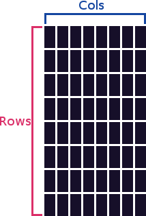
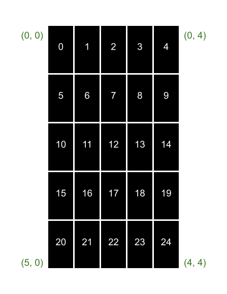
The tuple representing a position on the cell is (R, C) and not (C, R) -- where R represents a row and C a column. This is because terminals were designed to print text top to bottom, left to right. The origin (0, 0) is at the top left of the terminal window:

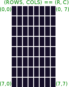
Note: The screen above is a square cell, but terminals and fonts are not square, thus a square cell renders a rectangular shape.

Preparation and Cleanup

The code provided in the common.s file calls two GLIR functions. One before the visualizer is called, and one after.

1. GLIR_Start: This function must be called before the visualizer to prepare the terminal for the visualizer:
   • Resizes the screen to the user-specified size.
   • Hides the terminal cursor.
   • Clears the terminal to the default background color.
2. GLIR_End: This function must be called after the visualizer to revert the terminal back to its default state:
   • Resizes the screen back to default (24x80).
   • Shows the terminal cursor.
   • Clears all the previous terminal output.

Colours

For colours, GLIR uses the ANSI escape codes, which are a set of codes that can be used to change the color of the text or background of the terminal. GLIR abstracts away these ANSI escape codes and allow the user to simply select the desired color code from a 256-color lookup table:

Environment

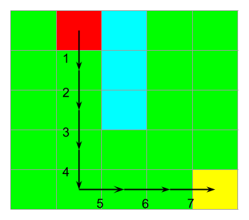
In this lab, you will implement and run A* on maps composed of $m\times n$ equally-sized cells, where $m$ is the number of columns and $n$ is the number of rows. It is guaranteed that $2\le m\le 32$ and $2\le n\le 32$ . Each cell can either be a grass cell (green), the start (red), the goal (yellow), or a water cell (light blue). Each cell is associated with a unique non-negative integer, or cell number. The uppermost left cell is numbered 0, and increments by one each time we move one cell to the right. If we reach the end of the row, we wrap to the left most cell one row below, and continue.

From any cell, we can only move into a cell that is immediately to the left, right, top, and bottom with a distance of one (1) unit (we will call these the adjacent cells). We cannot move into a water cell, nor can we move off the map.

Below is a picture illustrating the environment:

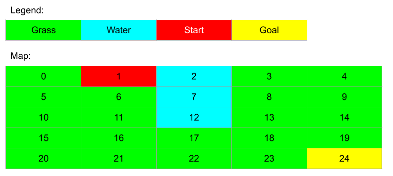
From cell 1, we can move into cells 0, and 6. We cannot move up because we will move off the map; we cannot move into cell 2 because it is a water cell; and we cannot move into cell 5 because it is diagonal from cell 1.

Paths

In this environment, paths are defined between two cells. Paths must obey the environment constraints described above. That is, a path is valid if all the cells on the path are grass cells, and, informally, you can trace the path with a pen from start to finish without lifting your pen, and without crossing into diagonal cells. For example:

Path Concepts

Path Representation

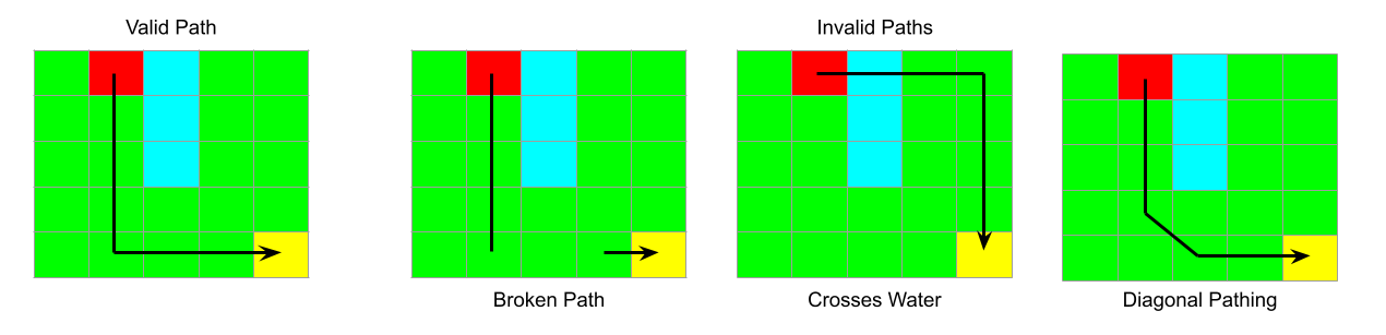
A valid path can also be represented as a sequence of cell numbers of the cells that makes up the path. For example, the valid path in the image above can be represented as 1, 6, 11, 16, 21, 22, 23, 24 , which means that the path starts at cell 1, goes through cells 6, 11, 16, 21, 22, 23 (in that order), and terminates at cell 24.

Distance

In the environment for this lab, the distance between adjacent cells is one (1) unit. The distance of a path is defined to be the distance between the first cell and the last cell of the path. For a path with $n$ cells, we have to move $n-1$ times to travel from the first cell to the last cell on the path. Therefore, the distance for a path with $n$ cells is $n-1$ units.

For example, there are eight cells in the path shown in the image below: 1, 6, 11, 16, 21, 22, 23, 24, and its distance is $8-1=7$ units.

A*

Terminology

This section introduces A* in the context of the environment described above, and also introduces some A* terminology.

• In a path $P$ from the start cell to an arbitrary cell $A$, the parent of $A$ is another cell $B$ that comes immediately before $A$ on $P$. $A$ is a child of $B$.
  • The parent of the start is defined to be itself.
• Given a valid path $P$ and a cell $A$ in $P$, the g of $A$ is the distance from the start to $A$ in $P$.
• The h of $A$ is the estimated distance from $A$ to the goal. A heuristic function is used to estimate this value.
• f := g + h.

To store information, A* uses two lists:

• A closed list that stores the parent, g, and h of each cell that has been expanded.
• An open list that keeps track of the cells that have been visited but not yet expanded.

There are many ways to implement the closed list and the open list. In a later section, we will detail how they should be implemented in this lab.

Algorithm

The previous section assumed that A* has already found a valid path from the start to a cell $A$. This section lifts this assumption to discuss how A* actually finds such valid paths.

The search begins with A* recording the parent, g, and h for the start cell. The parent of the start cell is defined to be itself, thus g is zero. The h of a cell is computed by an heuristic function. After A* has recorded the parent, g, and h for the start cell, the start cell has been visited. A* now visits the adjacent cells of the start cell, setting their parent as the start cell, their g as one, and their h computed using the heuristic function. After visiting all the adjacent cells of the start cell, the start cell is considered expanded. A* continues to expand visited cells until it expands the goal, in which case a solution path is found, or when there no more visited cells to expand, in which case no solution paths are found.

A* prioritizes expanding cells with the shortest estimated path from the start to the goal by expanding the cell with the smallest f first. Open List details how to efficiently find the cell with the smallest f among all the visited cells.

There can be multiple paths from the start cell to a cell $A$. Thus, there migh be multiple parents and values of g for $A$. The Closed List of A* keeps only the parent and g of $A$ for the shortest path from the start to $A$.

Below is the pseudocode for A*:

A* Search
Initialize the open list
Initialize the closed list
Visit the start cell
Insert the start cell into the open list
while the open list is not empty
  let $q$ be the cell with the least f
  pop $q$ from the open list

  if $q$ is the goal
    stop the search

  Redraw the cell corresponding to $q$ with the color gray

  // Expand $s$
  generate all 4 adjacent cells of $q$
  for each adjacent cell, $s$, of $q$
    if $s$ is a water cell or $s$ is off the map
      skip $s$
    else
      $s$.parent = $q$

      // dist(start,$s$) = dist(start,$q$) + dist($q$,$s$)
      // In our environment, dist($q$, $s$) = 1
      $s$.g = $q$.g + dist($q$, $s$)

      // Estimate the distance from $s$ to $\mathrm{goal}$
      $s$.h = heur($s$, $\mathrm{goal}$)

      // We have not explored $s$ yet
      if $s$ is not in closed list
        add $s$ to the closed list
        (closed list).$s$.parent = $s$.parent
        (closed list).$s$.g = $s$.g
        (closed list).$s$.h = $s$.h
        add $s$ to the open list
        Check and maintain heap property of the open list

      // We have found a shorter path to $s$
      if $s$ is in the closed list AND $s$.g < (closed list).$s$.g
        update $s$.parent, $s$.g, and $s$.h in the closed list
        Check and maintain heap property of the open list
end A* Search
      

The part in the pseudocode that is highlighted in yellow draws updates of the map to the terminal. Updating the terminal is discussed in detail here. The parts in the pseudocode that is highlighted in green will be explained in a later section.

The Pathfinder

Exploration

This lab requires that your implementation of A* visits adjacent cells in the following order: left, right, top, and bottom.

Building the map

In this lab, the internal representation of the entire map is stored in the map buffer. The map buffer is an 1D array of 32-bit integers where the $i$'th element of the array contains the value 1 if the $i$'th cell is a water cell and it contains the value 0 otherwise. The common.s file pre-allocates the map buffer and passes the pointer to the map buffer as an argument to the student's pathFinder procedure.

Another argument to the pathFinder procedure is a pointer to the water array. The water array is an array of 32-bit integers where each integer is the cell number of a water cell in a particular map. The cell numbers in the water array are not guaranteed to be sorted in any particular order.

Closed List

This lab implements the closed list as an 1D array of structures, described below. The common.s file pre-allocates enough space for each cell to have an entry in the closed list, and will pass the pointer to the closed list as an argument to the student's pathFinder procedure. Each entry in the array will be a struct containing three 32-bit integers in the following order: parent, g, h. For simplicity, the cell number of a cell and the index of its corresponding entry in the closed list must be the same (e.g. the corresponding entry of cell 7 should have an index of 7 In the closed list). Your code must initialize the open and closed lists before running the A* algorithm. This initialization is described in this section.

A parent of -1 indicates that the cell has not been visited yet. If a cell has been visited, the solution must record its parent, g, and h in the corresponding entry of the cell. The parent and g of a cell must be updated whenever A* finds a shorter path to the cell than the current known path.

The image below summarizes the in-memory representation of the map buffer, the water array, the closed list, and the open list.

Open List

The open list keeps track of the cells that are visited but that are not expanded yet. As seen in the A* pseudocode, A* does this by adding a cell to the open list whenever it visits the cell for the first time, and removing a cell whenever it expands the cell. In every iteration of the search, A* expands one cell, and visits a maximum of four cells. Hence, operations such as insertion and deletion from the open list needs to be efficient. For this reason, this lab implements the open list using a min-heap.

(Min-)Heap

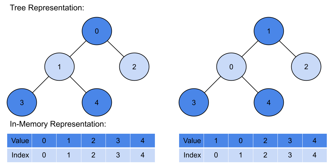
The heap data structure is a complete binary tree that satisfies the heap property. In memory, this lab represents such a binary tree using an 1D array of 32-bit integers, where the root node has an index of zero. For any given node in the tree with index $i$, its left child has an index of $2\times i+1$, and its right child has an index of $2\times i+2$. For the binary tree to satisfy the heap property of a min-heap, the root node must have the smallest key, and, for any given node, its key must be less than or equal to the key of its children (if any). The key is simply a value used to order the entries in the heap. In this lab, the entries in the heap are cell numbers, and the keys are the f value of the cells.

The image below shows two trees with their respective in-memory representation directly below their tree representation. The number inside the tree nodes are keys. The tree on the left satisfies the min-heap property while the tree on ther right does not because the key of its root node is greater than the key of its left child.

Heap Operations

The heap property must be checked for every insertion, deletion, or change of the key of an element. If the heap property no longer holds after a change, the heap must re-arrange the elements such that the heap property holds again (this action is called heapifying the tree/array). This requirement is highlighted in green in the A* pseudocode above.

The file heapq.s provides code for following heap operations that should be used for the solution for this lab:

• insert:
  • Arguments
    • a0: pointer to the open list
    • a1: pointer to the closed list
    • a2: the cell number of the cell to insert
  • Return
    • None
  • Effect
    • Inserts the cell with cell number given by a2 into the open list. Maintains the heap property based on the f values of the cells.
• popMin:
  • Arguments
    • a0: pointer to the open list
    • a1: pointer to the closed list
  • Return
    • a0: The cell number of the cell with the least f value in the open list
  • Effect
    • Removes the cell with the least f value from the open list and returns its cell number. Maintains the heap property based on the f values of the cells.
• minHeap:
  • Arguments
    • a0: pointer to the open list
    • a1: pointer to the closed list
  • Return
    • None
  • Effect
    • Transforms the array given by a1 into a heap in place based on the f values of the cells.

Although having a high-level understanding of the heap data structure and the heap operations is sufficient for students to complete the lab, it is strongly recommended that students take a look at heapq.s and try to understand the RISC-V implementation of the heap data structure and the heap operations.

Initialization

common.s passes the pointers to the map buffer, the open list, and the closed list to pathFinder as arguments. Sufficient space is allocated for each array, but the three arrays are not initialized. You must initialize the the open list and closed list in your aStar function as follows:

• Each element in the closed list is initialized as -1, 0, 0.
• To initialize the open list, simply set the size of the open list to zero (see Global Variables).

Heuristic function

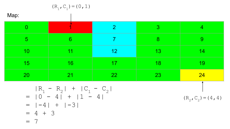
A heuristic function estimates the distance to go between a given cell and the goal. In this lab we will use the Manhattan distance as the heuristic function. The Manhattan distance measures the sum of the absolute differences between the coordinates of two points. As described in Drawing the map we can identify each cell with a tuple (R, C). The Manhattan distance between two cells is defined as: $$h = | R₁ - R₂ | + | C₁ - C₂ | . In other words, it is the absolute difference between the row numbers plus the absolute difference between the column numbers. The image below demonstrates the calculation of the Manhattan distance between cells 1 and 24 on a 5-by-5 map.

Drawing the map using GLIR

As mentioned here, each cell in the map is represented with a unique integer. GLIR however, prints to terminal using rows and columns. For the convenience of converting between the two systems of representation, align cell 0 with the cell located at (0, 0) on the terminal window.

In this lab all grass cells will be colored green, all water cells will be colored blue, the start will be colored red, and the goal cell will be colored yellow. Use color code 10 for green, color code 14 for blue, color code 9 for red, and color code 11 for yellow.

During the search, color any expanded node in grey. If a solution is found at the end of the search, you must color the solution path with purple. Use color code 8 for grey and color code 13 for purple.

Displaying Updates

There are multiple ways to display updates on the screen. This lab uses the following method:

1. Print the initial map (grass, start, goal, and water) onto the terminal.
2. As A* expands cells, redraw the corresponding cell in the terminal with the color gray.
3. If a solution path is found at the end of the search, trace the solution path backwards from the goal, and recolor each cell on the path with purple. If no solutions are found, then nothing needs to be done.
4. Redraw the start and goal cells.

All the steps can be achieved using the GLIR_PrintRect subroutine.

GLIR_PrintRect

Below is the function specification of the GLIR_PrintRect method is the GLIR library.

GLIR_PrintRect

Arguments:
  a0: Row of the top left corner
  a1: Col of the top left corner
  a2: Signed height of the rectangle
  a3: Signed width of the rectangle
  a4: Color to print with
  a5: Address of null-terminated string to print with; if 0 then uses
      the unicode full block char (█) as default

Returns:
  None

Prints a rectangle using the (Row, Col) point as the top left corner having
width and height as specified. Supports negative widths and heights.
Specifying a height and width of 0 will print a rectangle one cell high by
one cell wide.
      

To draw the initial map, we recommend that you use the GLIR_PrintRect method to draw the cells of the map one by one. You can redraw a cell with a different colour by calling the GLIR_PrintRect method with the coordinates of the cell and the desired colour.

Putting Everything Together

Here is the general flow of the visualizer.

1. Build the map. See Building the map.
2. Draw the map on the terminal. See Drawing the map and Color of cells.
3. Run A* search from the start.
4. If a solution path is found, draw the solution path in purple.
5. Redraw the start and the goal cells.

The video below is a short demonstration of how the map, and the states of the closed list and the open list changes as A* searches the environment. This video is created by screen recording slides 47-60 in the presentation for this lab.

Example Output

When testing, provide the map specification file as program arguments using the pa commandline option of the RARS simulator. For example: rars pathFinder.s pa test-map-1.txt

This output has been slowed down on purpose. The speed of the animation in the example output may not match your output. This is perfectly fine as the speed of the animation will vary depending on the speed of your computer and operating system.

Global Variables

We define the following global variables in common.s:

• ROWS: the number of rows in the map
• COLS: the number of columns in the map
• GREEN: the color code for green
• BLUE: the color code for blue
• YELLOW: the color code for yellow
• RED: the color code for red
• GREY: the color code for grey
• PURPLE: the color code for purple

heapq.s also provides the current size of the heap (open list) as a global variable:

• SIZE: the size of the open list

Input Guarantees

• All maps will have at least 2 rows/columns, and at most 32 rows/columns.
• commons.s will always set the dimension of the terminal to be the same as the dimension of the input map.
• The map buffer, closed list, and open list are guaranteed to be large enough for maps up to the maximum size of 32 rows by 32 columns.
• The input file is guaranteed to have the dimension of the map, the start and the goal. i.e. students are not required to check for missing inputs.
• The size of the input file is guaranteed to be at most 2048 bytes.

Specifications

The solution must follow the RISC-V register saving/restoring calling conventions .

The solution for this lab is implemented in pathFinder.s. which must implement the following functions:

• pathFinder:
  • Arguments
    • a0: pointer to the open list
    • a1: pointer to the closed list
    • a2: pointer to the map buffer.
    • a3: the cell number of the start cell
    • a4: the cell number of the gaol cell
    • a5: pointer to the water array.
    • a6: length of the water array
  • Return Values:
    • a0: 1 if a solution path is found, 0 otherwise.
  • Effect:

    This is the entry point of the pathfinding visualizer. This method should:

    1. Build the map
    2. Draw the map on the terminal
    3. Run A* search from the start
    4. If the solution path is found, draw the solution path on the terminal
    5. Redraw the start and goal cells
  • Note:
    • See Visualizing the Search
• buildMap:
  • Arguments:
    • a0: pointer to the water array.
    • a1: length of the water array
    • a2: pointer to the map buffer
  • Return Values:
    • None
  • Effect:
    • Construct a 1D array such that the $i$'th element of the array is a 1 if the $i$'th cell is a water cell and a 0 otherwise.
• drawMap:
  • Arguments:
    • a0: pointer to the map buffer.
    • a1: the cell number of the start cell
    • a2: the cell number of the goal cell
  • Return Values:
    • None
  • Effect:
    • draws the map to the terminal.
• aStar:
  • Arguments:
    • a0: pointer to the open list.
    • a1: pointer to the closed list.
    • a2: pointer to the map buffer
    • a3: the cell number of the start cell
    • a4: the cell number of the goal cell
  • Return Values:
    • a0: 1 if a solution path is found, 0 otherwise.
  • Effect:
    • Searches for a path from the start to the goal, coloring all the expanded nodes in gray.
  • Note:
    • See pseudocode here
• drawSoln:
  • Arguments:
    • a0: pointer to the closed list.
    • a1: the cell number of the start cell.
    • a2: the cell number of the goal cell.
  • Effect:
    • Draws the solution path on the terminal. This function should not do anything if no solution path was found. However, it should always redraw the start and goal cell.
• isWater:
  • Arguments:
    • a0: pointer to the map buffer.
    • a1: the cell to check
  • Return Values:
    • a0: 1 if the cell is a water cell, 0 otherwise.
  • Effect:
    • Checks if the given cell is a water cell or not.

• manhattan:
  • Arguments:
    • a0: the cell number of cell A
    • a1: the cell number of cell B
  • Return Values:
    • a0: the Manhattan distance between cell A and cell B
  • Effect:
    • Calculates the Manhattan distance between two cells, A and B

Testing

Testing the Non-Visual Functions

This is a visual lab. Thus, it may be difficult to test the non-visual functions: buildMap, isWater, and manhattan. These functions are tested automatically by common.s when you run pathFinder.s.

Running the Visualizer

• Linux and macOS: Using the terminal, navigate to the directory containing your code, then run rars pathFinder.s pa <map-spec-file.txt>.
• Windows: Using a lab machine running on the Windows PowerShell or Command Prompt terminal, navigate to the directory containing your code, then run rars pathFinder.s pa <map-spec-file.txt>.
  • Note: GLIR is not supported on Windows Terminal. If you are using Windows, you must use the Command Prompt or Windows PowerShell native terminal, not Windows Terminal, running one of the lab machines. You can do this by running either of them in Administrator mode.
  • Here are the steps to run the program in Windows:
    1. Search for "Command Prompt" or "Windows Terminal" through Windows Search.
    2. Right-click on "Command Prompt" or "Windows Terminal" and select "Run as Administrator". This will open their own terminal window.
    3. ssh into a lab machine. Instructions to access the lab machines can be found here. Follow the Linux/macOS instructions.
    4. Navigate to the directory containing your code and run rars pathFinder.s pa <map-spec-file.txt>.
  • Instructions of how to run the program in Windows PowerShell can be found in this video. The video was created for a different lab, but the general procedures are the same.
• As a last resort, use X2Go

Testing with Different Maps

We provide a Python script (<REPO_ROOT>/map-builder-tool/map_builder.py) that allows you to interactively create maps to test your solution. To use the tool, cd into the map-builder-tool directory and install the required packages: pip install -r requirements.txt. You can then run the tool by executing python3 map_builder.py, and follow the instructions in the program to create maps interactively.

When you click on the "Get Input File" button in the program, it generates a file with the following format:

ROWS COLS
START GOAL
the cell number of the water cells (if any) separated by whitespaces

      

For example, the following input file:

5 5
0 4
2 7 12 17

      

represents a map that has 5 rows and 5 columns, where cell 0 is the start, cell 4 is the goal, and cells 2, 7, 12, and 17 are water cells. Input files must have the empty line at the end of the file. commons.s will otherwise throw an 'Invalid file contents' error.

The "Get Input File" button will also print the location of the input file to the terminal that you used to launch the program. Please also refer to the same terminal for other program messages.

Here is a sample execution of the map builder tool on an Intel machine running Debian 12 with GNOME 43.9 as the desktop environment:

Resources

• Class slides used for this lab (.pptx) (.pdf).
• Read more about GLIR here (GLIR).
• The API reference of GLIR can be found here (GLIR Reference).
• Marksheet used to mark the lab (.txt)

Notes and Tips

• Start with implementing the non-visual functions as we provide testcases and expected outputs for those functions.
• You can then implement drawMap and test it using the map builder tool.
• Implement aStar and drawSoln last.
• Test your program with different maps by generating map input files using the map builder tool.

Marking Guide

Assignments too short to be adequately judged for code quality will be given a zero.

• 26% for correct visual output of drawMap, A*, and drawSoln.
• 20% for correct overall visual output.
• 18% for correct buildMap, isWater, and manhattan procedures.
• 15% for correct A* algorithm.
• 1% for correct a0 return value from the pathFinder procedure.
• 20% for code cleanliness, readability, and comments.

Submission

Ensure that your solution works in the lab machines because it will be graded using the lab machines.

There is one file to be submitted for this lab:

• pathFinder.s should contain the code for A* search and visualizing the map. You can add additional functions as you see fit.
  • Do not add a main label to this file.
  • Do not modify the line .include "common.s".
  • Do not modify the common.s file.